📈 Monitoring#
The Monitoring module is divided into two sections—Data Drift Detectors and Model Divergence. Together, they allow you to monitor deployed soft sensors, interpret drift scores, and compare the performance of different models to support ongoing evaluation and decision-making.
Data Drift detectors#
The Drift Detectors section enables you to continuously monitor the performance of each soft-sensor model by analyzing how it behaves over time, based on the data associated with a selected experiment ID. It provides intuitive controls to adjust the time window and define the specific subset of data you want to evaluate.
Within this section, you can choose from the drift detection methods available in the STAMM dashboard. Each detector comes with its own metric and configurable parameters. Once you select a detector and set its parameters, STAMM computes the drift, displays the results, and provides a clear explanation of the detected behavior.
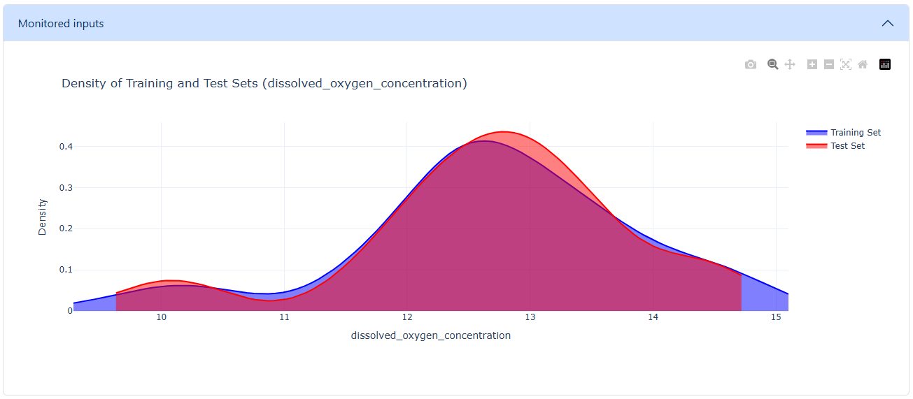
The dashboard also includes a density plot that compares the distributions of the training and test datasets for the specified data range. This visualization helps you assess distribution shifts and determine whether the model may be experiencing data drift.
Overall, the Drift Detectors section offers a straightforward and flexible way to detect drift, understand its potential causes, and assess the long-term stability of your models.
The following sections describe the different features and controls available here to help you use this functionality effectively.
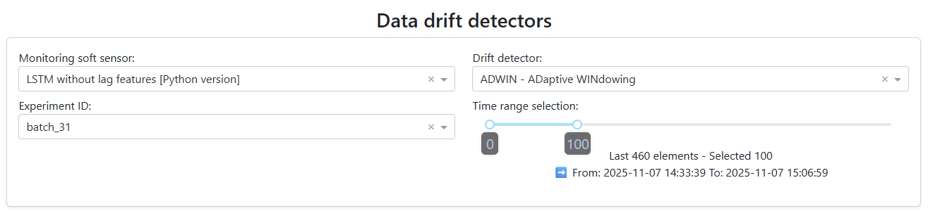
Select the soft-sensor model to analyze, choose the drift detector, specify the experiment ID that provides the data, and customize the amount of data to process. A slider is available to adjust the data window, which defaults to the most recent 100 data points.
Set the parameter values for the selected metric. Once you choose a metric in the previous step, the dashboard automatically loads the corresponding parameters. If the detector uses a univariate metric, the interface will also display a dropdown that allows you to select the specific variable to which the metric will be applied.
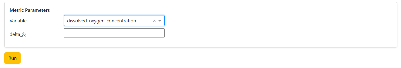
If you selected a multivariate metric, only the parameter fields will appear, since no variable selection is required.
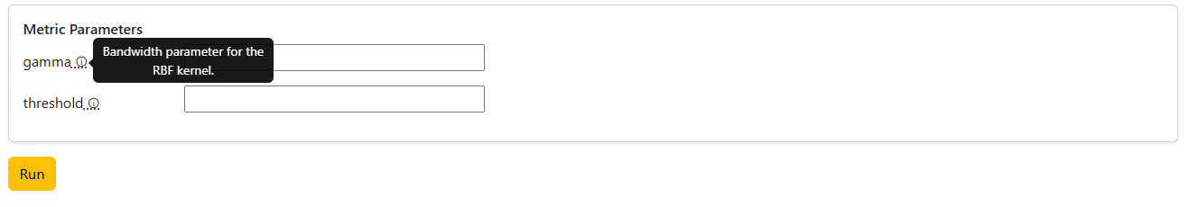
Each parameter field includes a tooltip that provides a brief description of its purpose.
After set all parameters, click Run to execute the detector and view the results.
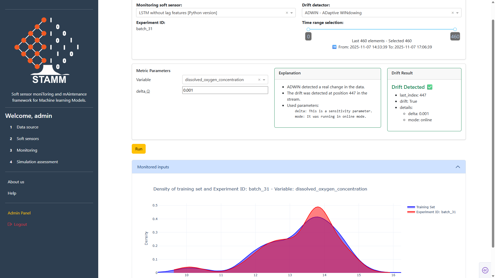
The drift detector results are displayed to the right of the metric parameters. The output is divided into two main components:
Explanation: A human-friendly summary that helps you interpret the result.
Drift Result: A more detailed breakdown of the detector’s output, including:
Index: The point at which drift was detected. A value of -1 indicates that no drift was found.
Drift: A boolean value (True or False) indicating whether drift is present.
Details: Additional information about the metric parameters used in the calculation.
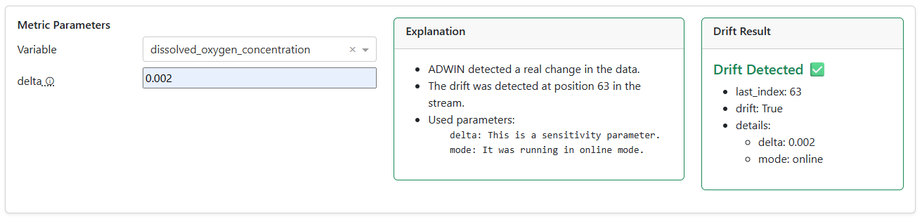
These elements work together to provide both a high-level interpretation and a precise technical view of the detector’s output.
In addition, the section displays a density plot that compares the distribution of the training data with the distribution of the analyzed (test) data. This visualization helps you quickly assess how closely the two datasets align and whether any distributional shifts may be contributing to drift
🎬 Video: Monitoring Drift and Model Stability
Discover how to use univariate and multivariate drift detectors to monitor deployed soft sensors, interpret drift scores, and explore train–test density comparison plots for data consistency validation.
Model divergence#
Another key subsection within Monitoring is Model Divergence, which provides a set of tools to compare the performance of the deployed soft-sensor model—configured in the Soft Sensors section and linked to the selected experiment ID in the Datasource section—against other models available in the Model Registry. The dropdown in this subsection pulls all registered models available, allowing you to easily select which ones you want to evaluate.
The Model Divergence view helps you visualize how alternative models behave relative to the deployed model and assess their overall alignment or deviation. In addition, it calculates a performance estimator that quantifies how each selected model performs when compared to the deployed baseline.
Overall, this subsection allows you to quickly identify performance gaps, explore potential improvements, and better understand the robustness of your deployed model in relation to other candidates in Model Registry.
The following points provide a clear explanation of the available functionalities and how to use them effectively.
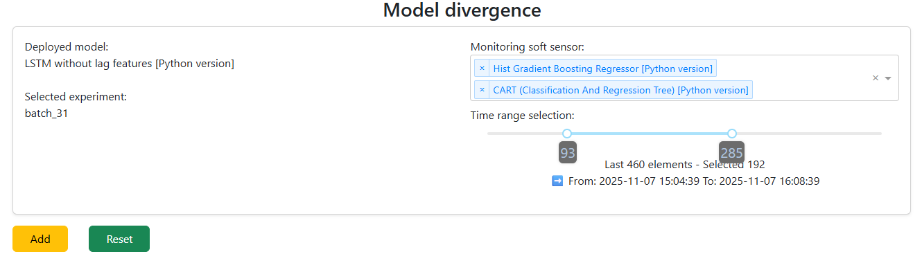
Select the models to analyze. This control automatically loads the deployed model defined in Soft Sensors and the selected experiment from the Data Source section. A dropdown displays all soft-sensor models available in the Model Repository, allowing you to choose one or multiple models to compare against the deployed baseline.
You can also customize the amount of data included in the comparison by adjusting the data window through a slider, giving you flexibility to focus on recent data or a broader historical range.
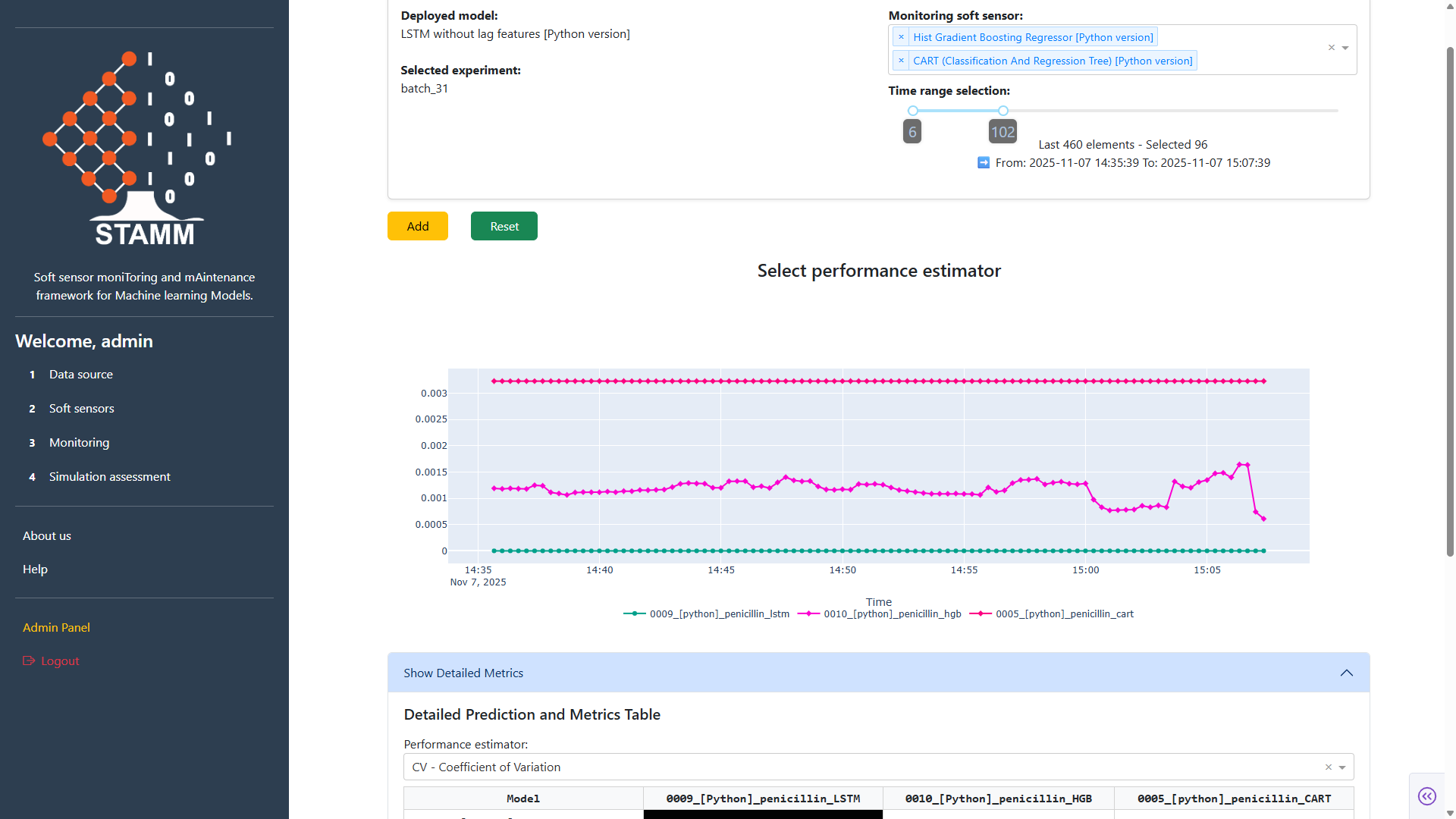
Once you have selected the models to monitor and defined the time window, clicking Add generates a performance visualization in the STAMM dashboard. This chart allows you to easily compare and analyze the behavior of the selected models within the chosen data range, helping you identify patterns, deviations, and overall performance differences.
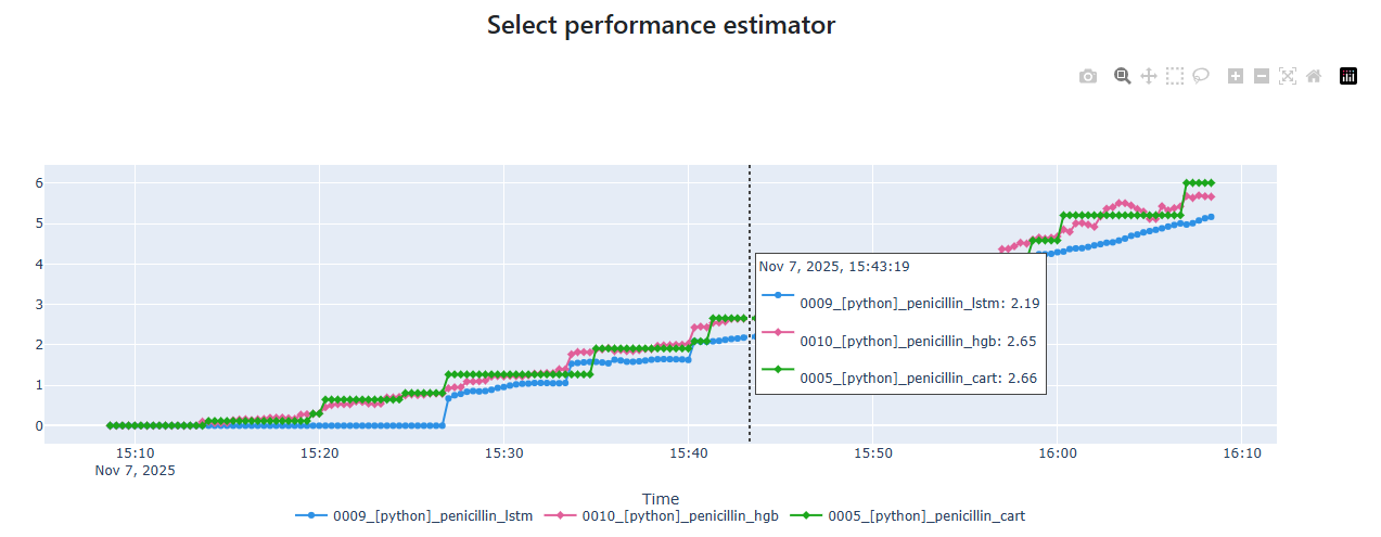
After selecting the models to monitor and defining the time window, clicking Add will also load a component in the STAMM dashboard that allows you to choose a performance estimator. This estimator evaluates how each selected model compares to the deployed model, using the deployed model as the baseline for all performance calculations.
The results of the selected estimator are presented in a matrix-style table, making it easy to compare models side by side and understand their relative performance.
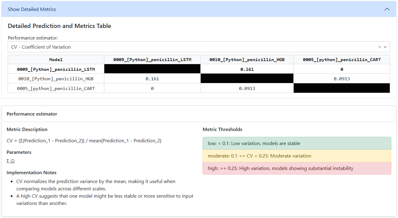
Each time you choose a performance estimator, the dashboard automatically displays a detailed information panel. This panel includes the estimator’s description, required parameters, implementation notes, and recommended thresholds, providing you with all the context needed to configure and interpret the estimator effectively.
🎬 Video: Model Divergence and Comparative Evaluation
Learn how to use the Model Divergence tools to compare the deployed soft-sensor model with alternative candidates from the Model Registry, visualize their relative behavior, and interpret the performance estimator that quantifies how each model aligns with—or deviates from—the deployed baseline.