Industrial-scale fermentation
🧫 Industrial-scale fermentation
To showcase what STAMM does on a realistic industrial process, we use a 100,000 L fed-batch fermentation for the production of penicillin by Penicillium chrysogenum as the reference case study. Data come from the open IndPenSim benchmark.
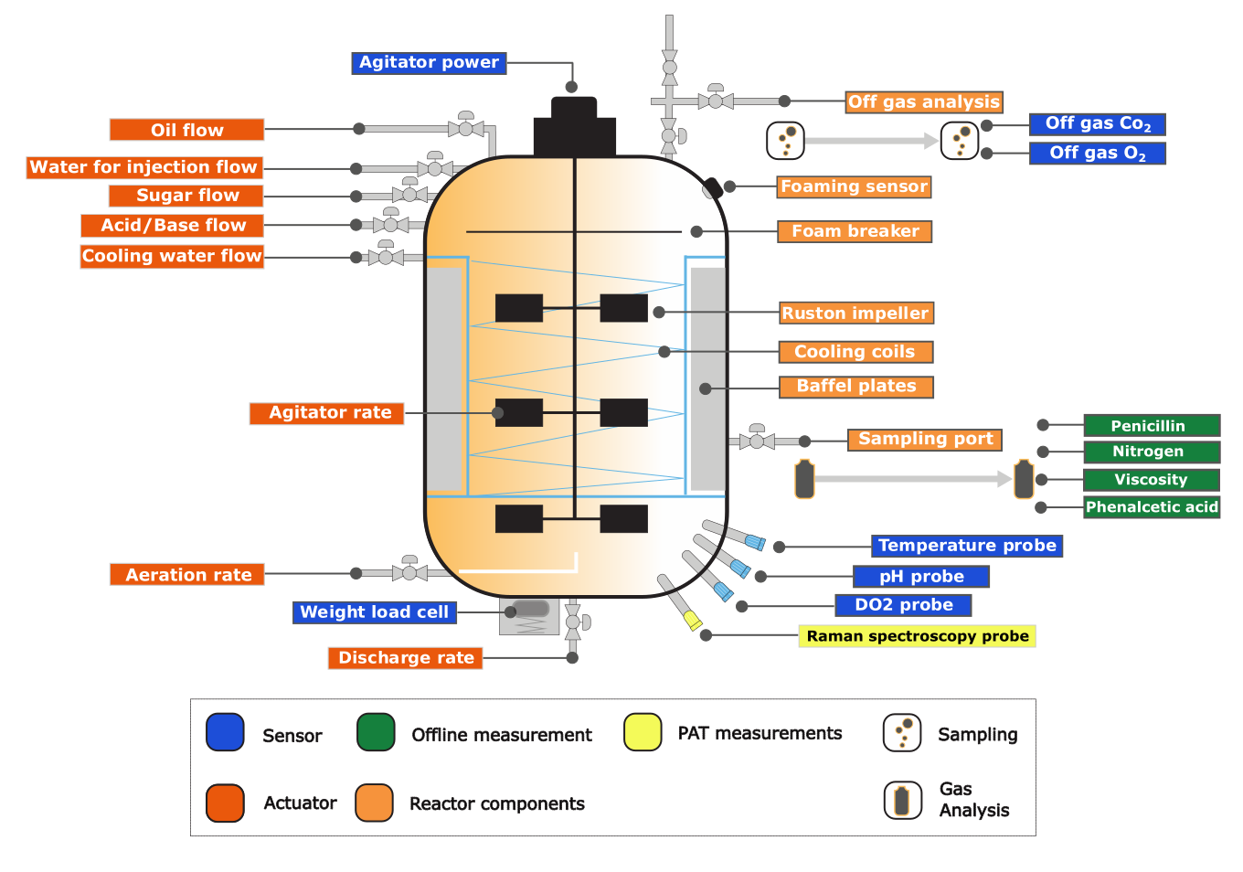
Why this case study
This type of large-scale fed-batch fermentation is representative of real industrial biotechnology operations, where process dynamics are nonlinear, measurements are noisy or delayed, and supervisory control must be combined with advanced monitoring and optimization strategies. It's the kind of setting where soft sensors actually earn their keep — and where STAMM's monitoring and maintenance layer matters.
The data originate from the Industrial Penicillin Simulation dataset (IndPenSim) — a first-principles benchmark model and open dataset that replicates an industrial penicillin campaign in silico, capturing the dynamics, noise, and operating regimes you'd encounter on a real plant. The benchmark comprises 100 batches produced under three control strategies — recipe-driven (batches 1–30), operator-controlled (31–60), and advanced process control with Raman spectroscopy (61–90) — with the final ten batches (91–100) containing faults and process deviations. This mix of slow non-stationary dynamics, heterogeneous control, and deliberately faulty batches is exactly the regime STAMM was designed for.
Seven soft sensors, one endpoint
To demonstrate that the model registry is genuinely language- and learner-agnostic, seven soft sensors that predict penicillin concentration (P) were registered and deployed together. Four are the interpretable learners from Acosta-Pavas et al. (2024) — CART, M5, CUBIST, and Random Forest — originally built in R; CART and Random Forest were additionally re-implemented in Python. Three more black-box models — a Support Vector Machine (SVM), a Gradient Boosting Machine (GBM), and a Long Short-Term Memory network (LSTM) — were trained on the same 80:20 batch split. Despite their architectural and language differences, all seven are served through the same REST /predict endpoint.
The table below reports each soft sensor's predictive performance on the held-out test set (from the STAMM paper). The best black-box model (LSTM) and the best interpretable model (CUBIST) are separated by less than one percentage point in R² and about 0.08 in MAE — close enough to share an operating regime, which is precisely what makes the framework's output-level model-divergence signal informative.
| Model | Type | Language | R² | MSE | RMSE | MAE |
|---|---|---|---|---|---|---|
| CART | Interpretable | R / Python | 0.775 | 24.061 | 4.905 | 3.328 |
| M5 | Interpretable | R | 0.777 | 23.823 | 4.880 | 3.221 |
| CUBIST | Interpretable | R | 0.908 | 9.916 | 3.149 | 1.920 |
| RF (Random Forest) | Interpretable | R / Python | 0.905 | 10.202 | 3.194 | 1.928 |
| SVM | Black-box | Python | 0.847 | 16.107 | 4.013 | 2.317 |
| GBM | Black-box | Python | 0.904 | 10.146 | 3.185 | 1.930 |
| LSTM | Black-box | Python | 0.916 | 8.800 | 2.966 | 1.843 |
Bold values mark the best score within each learner family (interpretable vs. black-box) for every metric. Results for the interpretable learners and the train/test split follow Acosta-Pavas et al. (2024).